Profiling Example
Overview
This example illustrates the use of the various profiling tools and APIs available on the Hexagon SDK. This example also measures and reports the FastRPC performance with different buffer sizes and optimizations.
This example shows how to use the following:
- The FastRPC performance tests can be viewed in the shell. These tests print the overhead time for a CPU thread to offload a task to the DSP, wait for the DSP to execute that task, and wake up when the task is complete. The time measurements are meaningless on the simulator.
- The timer APIs demonstrate the APIs that can be used for accessing cycle and clock counters and use them to time a block of code. These APIs work on both the simulator and device. The time measurements are meaningless on the simulator.
- The Hexagon Profiler generates function-level profiling reports. This profiler can be used only on the simulator.
- The Hexagon Trace Analyzer parses trace files generated on device or on simulator and generates various analysis reports. This profiler works only on Linux.
- The sysMonApp displays various performance-related services on the cDSP, aDSP, and sDSP. This profiler can only be used on device.
Prerequisites
Before the profiling application is run the following conditions should be met:
- Make sure the Hexagon SDK is properly setup with the Setup Instructions.
- Some of the profiling tools discussed in this example are not supported on all devices. Please refer to the feature matrix for more details.
- Access to a browser with internet, preferably Chrome.
- This will allow use of Perfetto viewer to view the traces generated by the Hexagon Trace Analyzer
- The Hexagon Trace Analyzer requires Flamegraph. This tool will be downloaded from the internet when the run_profilers.py script is run for the first time. You can download Flamegraph here.
- The Windows version of Hexagon Trace Analyzer requires Perl to be installed. You can download Perl here.
Running profiling_walkthrough.py
The profiling_walkthrough.py script builds and runs the timer APIs and default FastRPC performance tests on a device.
Usage: profiling_walkthrough.py [-p] [-n ITERATIONS] [-i] [-m] [-u] [-Q FASTRPC_QOS] [-q FASTRPC_QOS_LATENCY] [-U UNSIGNED_PD_FLAG]
In addition to the options supported by all walkthrough scripts, the profiling_walkthrough.py script supports the following options:
- Optional arguments:
| Option | Description | Default |
|---|---|---|
| -n ITERATIONS | Number of iterations to run. | -n 1000 |
| -d DOMAIN | Specifies the domain on which to run the example. MDSP and SDSP are not supported. Domain is CDSP by default. 0: ADSP 3: CDSP | -d 3 |
| -Q FASTRPC_QOS | Set the FastRPC QoS mode. This can improve performance at the expense of some increase in power consumption. PM(Power Manager) QoS (mode 1) by default. 3 enables poll QoS and 0 turns QoS OFF. | -Q 1 |
| -q FASTRPC_QOS_LATENCY | Set the latency or the timeout of FastRPC QoS mode in microseconds. If fastrpc_qos is PM QoS (1), set the latency of PM QoS. If fastrpc_qos is Poll QoS (3), set the timeout of Poll QoS. | -q 300 for PM QoS, -q 1000 for Poll QoS |
| -y SLEEP_LATENCY | Set DSP Sleep Latency. 0 is default and means DCVS V3 vote will not be made. Range of values is from 10 to 65535 microseconds. To remove a previous latency vote, simply vote for a large latency such as 65535 to indicate that there is no specific latency request. | -y 0 |
| -U UNSIGNED_PD_FLAG | Set the PD to run the example. 1 is default and means run the example on the Unsigned PD. | -U 1 |
| -p | Run power boost using the request type HAP_power_set_DCVS_v3 with HAP_DCVS_V2_PERFORMANCE_MODE. Further details are provided below. | OFF |
| -i | Disable ION memory for FastRPC performance tests. ION memory is used by default. This option is relevant only for FUNCTION_NAME default, noop, inbuf, routbuf. Otherwise this option is ignored. | ON |
| -m | Verify memory operations for FastRPC performance tests by passing a fixed pattern to the DSP function which copies it to the output. The caller then confirms the correct pattern is received. | OFF |
| -u | Use uncached buffers on the HLOS. | OFF |
| -r | Manage ETM Capture programatically. | OFF |
For example, to build and run the timer APIs and default FastRPC performance tests on a Lahaina device:
python profiling_walkthrough.py -T lahaina
Building
Before modifying or understanding the code, we need to make sure we can build the example and generate the binary files from source. You can reproduce the steps of the walkthrough script by building and running the example manually as explained below.
- Build Android variant as follows:
make android BUILD=Debug - Build Hexagon variant as follows:
make hexagon BUILD=Debug DSP_ARCH=v65
For more information on the build flavors available and build syntax, please refer to the building reference instructions.
Running on device
- Use ADB as root and remount system read/write
adb root adb wait-for-device adb remount - Push Android components as follows:
adb wait-for-device shell mkdir -p /vendor/bin adb wait-for-device push android_Debug_aarch64/ship/profiling /vendor/bin adb wait-for-device shell chmod 777 /vendor/bin/profiling adb wait-for-device push android_Debug_aarch64/ship/libprofiling.so /vendor/lib64/ - Push Hexagon components as follows:
adb wait-for-device shell mkdir -p /vendor/lib/rfsa/dsp/sdk/ adb wait-for-device push hexagon_Debug_toolv87_v66/ship/libprofiling_skel.so /vendor/lib/rfsa/dsp/sdk/ - Generate a device-specific test signature based on the device serial number Follow the steps listed in the signing documentation.
NOTE: Signing the device needs to be done once as the same test signature will enable loading any module.
- Direct DSP messages to logcat:
adb wait-for-device shell "echo 0x1f > /vendor/lib/rfsa/dsp/sdk/profiling.farf" adb wait-for-device - Open another window to see aDSP diagnostic messages:
- Linux:
In a separate terminal:
adb logcat -s adsprpc -
Windows:
start cmd.exe /c adb logcat -s adsprpc sleep 2 -
Run Profiling Example:
adb shell "export LD_LIBRARY_PATH=/vendor/lib64/ DSP_LIBRARY_PATH=/vendor//lib/rfsa/dsp/sdk; /vendor/bin//profiling -f <function_name> -n <iterations> -s <size> -Q <fastrpc_qos> -q <fastrpc_qos_latency> -d <domain> -U <0/1> -y <sleep_latency>" -
Optional Arguments supported by the binary when running the timer APIs and FastRPC performance:
Usage: /vendor/bin/profiling [-f FUNCTION_NAME] [-n ITERATIONS] [-s SIZE] [-Q FASTRPC_QOS] [-q FASTRPC_QOS_LATENCY] [-U UNSIGNED_PD_FLAG] [-p] [-i] [-m] [-u]
| Option | Description |
|---|---|
| -f FUNCTION_NAME | Specify which function to run. The supported values are as follows:
|
| -d DOMAIN | Specifies the domain on which to run the example. MDSP and SDSP are not supported. Domain is CDSP by default. 0: ADSP 3: CDSP |
| -n ITERATIONS | Iterations to run FastRPC performance tests. 1000 is default. This option is relevant only for FUNCTION_NAME noop inbuf, routbuf. Otherwise this option is ignored. |
| -s SIZE | Size of data buffer for FastRPC performance tests. If 0 is given the noop function will run. |
| -Q FASTRPC_QOS | Set the FastRPC QoS mode. This can improve performance at the expense of some increase in power consumption. PM(Power Manager) QoS (mode 1) by default. 3 enables poll QoS and 0 turns QoS OFF. |
| -q FASTRPC_QOS_LATENCY | Set the latency or the timeout of FastRPC QoS mode. If fastrpc_qos is PM QoS (1), set the latency of PM QoS. If fastrpc_qos is Poll QoS (3), set the timeout of Poll QoS. |
| -y SLEEP_LATENCY | Set DSP Sleep Latency. 0 is default and means DCVS V3 vote will not be made. Range of values is from 10 to 65535 microseconds. To remove a previous latency vote, simply vote for a large latency such as 65535 to indicate that there is no specific latency request. |
| -U UNSIGNED_PD_FLAG | Set the PD to run the example. 1 is default and means run the example on the Unsigned PD. |
| -p | Run power boost using the request type HAP_power_set_DCVS_v3 with HAP_DCVS_V2_PERFORMANCE_MODE. Further details are provided below |
| -i | Disable ION memory for FastRPC performance tests. ION memory is used by default. This option is ignored with the FUNCTION_NAME timers. Otherwise the option is relevant. |
| -m | Verify memory operations for FastRPC performance tests by passing a fixed pattern to the DSP function which copies the pattern to the output. The caller then confirms the correct pattern is received. This option is relevant only for FUNCTION_NAME inbuf, routbuf. Otherwise this option is ignored. |
| -r | This option allows the user to control ETM trace capture programatically. It uses the HAP_user_etm_enable and HAP_user_etm_disable APIs to control the section of trace to be captured. |
| -u | Use Uncached buffers on HLOS for FastRPC performance tests. This option is relevant only for FUNCTION_NAME inbuf, routbuf. Otherwise this option is ignored. |
- Example commands with optional arguments to run the FastRPC tests on a specific buffer:
adb wait-for-device shell export LD_LIBRARY_PATH=/vendor/lib64/:$LD_LIBRARY_PATH DSP_LIBRARY_PATH="/vendor/lib/rfsa/dsp/sdk\;/vendor/lib/rfsa/dsp/testsig;" /vendor/bin/profiling -f inbuf -n 5000 -s 8388608 -p -q 700
The above example command will run the FastRPC performance test on an input buffer of size 8 MB with power boost and FastRPC QoS set to 700 micro-seconds.
adb wait-for-device shell export LD_LIBRARY_PATH=/vendor/lib64/:$LD_LIBRARY_PATH DSP_LIBRARY_PATH="/vendor/lib/rfsa/dsp/sdk\;/vendor/lib/rfsa/dsp/testsig;" /vendor/bin/profiling -f default
The above example command will run the FastRPC performance tests with on cached buffers, with ion disabled, with check memory off. The buffer types and sizes run will be the following:
| Buffer type | Buffer size |
|---|---|
| noop | 0K |
| inbuf | 32K |
| routbuf | 32K |
| inbuf | 64K |
| routbuf | 64K |
| inbuf | 128K |
| routbuf | 128K |
| inbuf | 1M |
| routbuf | 1M |
| inbuf | 4M |
| routbuf | 4M |
| inbuf | 8M |
| routbuf | 8M |
| inbuf | 16M |
| routbuf | 16M |
The results of the above command is as shown in Profiling summary report.
NOTE: The HAP user ETM APIs HAP_user_etm_enable and HAP_user_etm_disable are present in the profiling example code and executed at runtime by default. The user may move the calls to another place to profile another section.
Moreover the user has to run adb wait-for-device shell /data/local/tmp/sysMonApp etmTrace --command etm --hap_etm_enable 1 --q6 cdsp prior to running the profiling example with the ETM capture flag enabled.
Running on simulator
-
When running the example on the Hexagon simulator, you need to use the
--timingoption for the cycle count to be accurate. The time measurements will not be meaningful. -
When running on the simulator, you need to pass both the arguments to the Hexagon simulator and to the test executable.
-
The arguments given to the executable are given in the previous section.
-
The simulator arguments are as follows:
| Simulator option | Description |
|---|---|
--mv* |
Simulate for a particular architecture version of Hexagon. E.g. -mv65. |
--timing |
Model processor micro-architecture with cache, multi-threading mode, and processor stalls as part of the simulation. This enables timing so that the simulation more accurately models the operation of the processor hardware. |
--simulated_returnval |
Cause the simulator to return a value to its caller indicating the final execution status of the target application. |
--usefs <path> |
Cause the simulator to search for required files in the directory with the specified path. |
--pmu_statsfile <filename> |
Generate a PMU statistics file with the specified name. See the SysMon Profiler for more information about PMU events. |
--help |
Prints available simulator options. |
- The Hexagon Architecture version for the -mv* flag can be selected based on the DSP architecture version from the following:
| DSP Architecture version | Simulator Flag |
|---|---|
| v65 | -mv65a_1024 |
| v66 | -mv66g_1024 |
| v68 | -mv68n_1024 |
As an example, here is how the profiling_q.so file might be run on the simulator:
cd $HEXAGON_SDK_ROOT/examples/profiling/
$DEFAULT_HEXAGON_TOOLS_ROOT/Tools/bin/hexagon-sim -mv65a_1024 --timing --simulated_returnval --usefs hexagon_Debug_toolv87_v65 --pmu_statsfile hexagon_Debug_toolv87_v65/pmu_stats.txt --cosim_file hexagon_Debug_toolv87_v65/q6ss.cfg --l2tcm_base 0xd800 --rtos hexagon_Debug_toolv87_v65/osam.cfg $HEXAGON_SDK_ROOT/rtos/qurt/computev65/sdksim_bin/runelf.pbn -- $HEXAGON_SDK_ROOT/libs/run_main_on_hexagon/ship/hexagon_toolv87_v65/run_main_on_hexagon_sim -- ./hexagon_Debug_toolv87_v65/profiling_q.so -f timers
FastRPC performance tests
The FastRPC overhead can be calculated for different buffer sizes. Below is the brief description of the tests that can be executed:
| Function | Description |
|---|---|
| noop | Makes a FastRPC invocation with no input and output buffers |
| inbuf | Makes a FastRPC invocation with one input buffer of varying buffer sizes ranging from 32K to 16M |
| routbuf | Makes a FastRPC invocation with one output buffer of varying buffer sizes ranging from 32K to 16M |
The input buffer and output buffer are defined in the IDL file inc/profiling.idl. To understand the in and rout parameters given in the idl file, please refer to the IDL documentation.
Contributing factors to FastRPC performance
Various factors impact the performance of FastRPC. Some of the relevant factors are described below. For a detailed explanation of these factors refer to the system performance documentation. The profiling application allows you to explore the impact of some of these factors.
-
ION buffers: ION buffers (available on Android targets) do not require extra copies of buffers when shared between the DSP and the CPU. Non-ION buffers will automatically be copied by FastRPC framework. The impact on performance can be observed in the FastRPC performance tests by using the -i flag to disable ION memory for the FastRPC performance tests.
-
Caches: The FastRPC driver takes care of maintaining cache coherency between CPU and DSP for shared buffers. When the -u flag is given for uncached buffers, RPCMEM_HEAP_UNCACHED is used. You can refer to the RPCMEM API to learn more. Caching should result in better performance, but this depends on the application.
-
FastRPC QoS: FastRPC offers a QoS API to enable users to select a FastRPC QoS mode between CPU application making the remote call and beginning of DSP method execution. Refer to remote_handle_control() and remote_handle64_control() defined at remote API. In the FastRPC performance tests, the user can select a FastRPC QoS mode by providing it with the -Q flag. The default mode is 1 (PM QoS mode). 3 enables poll QoS and 0 turns QoS OFF. User can set a FastRPC QoS latency or timeout by providing it with the -q flag. The default latency is set to 300 microseconds for PM QoS. The default timeout is set to 1000 microseconds for Poll QoS.
| Index | Mode | Description |
|---|---|---|
| 0 | RPC_DISABLE_QOS | The CPU enters the low-power mode after sending an invocation to the DSP |
| 1 | RPC_POLL_QOS (Default) | Control the CPU low-power modes based on RPC activity in 100ms window |
| 3 | RPC_POLL_QOS | After sending an invocation to the DSP, the CPU will enter polling mode instead of waiting for a glink response until the timeout is reached |
-
Sleep latency: The low power sleep modes of the DSP can be entered by setting the DSP sleep latency. The DCVS V3 power voting is done to set the DSP sleep latency. This is supported only on limited devices. The values set for this should be in the range of 10 to 65535 microseconds.
-
Powerboost: If the power boost is set, the following DCVS V3 voting is implemented:
HAP_power_request_t request = {0};
request.type = HAP_power_set_DCVS_v3;
request.dcvs_v3.set_dcvs_enable = TRUE;
request.dcvs_v3.dcvs_enable = TRUE;
request.dcvs_v3.dcvs_option = HAP_DCVS_V2_PERFORMANCE_MODE;
request.dcvs_v3.set_bus_params = TRUE;
request.dcvs_v3.bus_params.min_corner = HAP_DCVS_VCORNER_MAX;
request.dcvs_v3.bus_params.max_corner = HAP_DCVS_VCORNER_MAX;
request.dcvs_v3.bus_params.target_corner = HAP_DCVS_VCORNER_MAX;
request.dcvs_v3.set_core_params = TRUE;
request.dcvs_v3.core_params.min_corner = HAP_DCVS_VCORNER_MAX;
request.dcvs_v3.core_params.max_corner = HAP_DCVS_VCORNER_MAX;
request.dcvs_v3.core_params.target_corner = HAP_DCVS_VCORNER_MAX;
request.dcvs_v3.set_sleep_disable = TRUE;
request.dcvs_v3.sleep_disable = TRUE;
HAP_power_set(NULL, &request);
The above settings can be found in the src/rpcperf_imp.c: profiling_powerboost() and profiling_sleep_latency(). To understand the DCVS_v2 and DCVS_v3 APIs, please refer to the HAP_power API documentation.
NOTE: Please note the following when running the FastRPC performance tests:
- There may be variability of timing results between runs
- The variability of timing results could be attributed due to a few reasons:
- Workload on the system
- Some entity in the system may be entering or exiting low power modes.
- The variability of timing results could be attributed due to a few reasons:
- The noop operation is run once before running the FastRPC performance tests on the inbuf and routbuf buffers. This is done so as to ignore the additional overhead of starting a FastRPC session on the DSP. This noop operation is not a part of the average overhead time displayed.
- The default Linux kernel boot image enables some config items that would impact performance. The Linux kernel boot image should be built with perf defconfig.
- The average overhead time should be computed over many iterations, to be more accurate.
Profiling summary report
The FastRPC performance tests described above returns the following summary report on the command line. This report shows the average FastRPC overhead in microseconds when making FastRPC calls per iteration, with variable input and output buffer sizes.
NOTE: The average FastRPC overhead per iteration will vary depending on the target and other factors
adb wait-for-device shell export LD_LIBRARY_PATH=/vendor/lib64/:$LD_LIBRARY_PATH DSP_LIBRARY_PATH="/vendor/lib/rfsa/dsp/sdk\;/vendor/lib/rfsa/dsp/testsig;" /vendor/bin/profiling -f default
[Test_Name Buffer_Size]  Avg FastRPC overhead per iteration(micro-seconds)

[noop        0K]          311us
[inbuf      32K]          634us
[routbuf    32K]          627us
[inbuf      64K]          713us
[routbuf    64K]          784us
[inbuf     128K]          823us
[routbuf   128K]          790us
[inbuf       1M]          909us
[routbuf     1M]          887us
[inbuf       4M]          900us
[routbuf     4M]          891us
[inbuf       8M]          897us
[routbuf     8M]          907us
[inbuf      16M]          919us
[routbuf    16M]          896us
Running run_profilers.py
The run_profilers.py script can be used to run the following profiling tools on simulator and on device:
Unlike the profiling_walkthrough.py script, the run_profilers.py script does not automate the steps of building the binaries and running them on to the device. The user needs to ensure that the profiling_walkthrough.py script has been run or the binaries are present on the device.
Usage: run_profilers.py -T Target [-P] [-HS] [-HT] [-SA] [-A] [-c] [-S] [-E CUSTOM_EXAMPLE ["Custom Arguments"]]
- Required Argument:
| Option | Description |
|---|---|
| -T TARGET | Specify the TARGET on which to run the script. Can be any supported device in the feature matrix |
- Optional Arguments:
| Option | Description |
|---|---|
| -P | Run the Hexagon Profiler to profile an excutable running on the Hexgon Simulator |
| -HS | Run the Hexagon Trace Analyzer for Simulator to profile an executable running on the Hexagon Simulator |
| -HT | Run the Hexagon Trace Analyzer to profile an executable running on the selected device |
| -SA | Run the Sysmon App on a selected target device |
| -A | Run all the profilers sequentially on Hexagon Simulator and selected target |
| -c | Skip running the one_time_script.py for the Hexagon Trace Analyzer |
| -S | Enter a custom size for Trace buffer in Hexadecimal Format. Default is 0x40000000 i.e. 64MB |
| -E CUSTOM_EXAMPLE [ "CUSTOM ARGUMENTS" ] | Run the Hexagon Trace Analyzer on target for a custom example. The absolute path needs to be provided. It is assumed that the example has been succesfully built and that the binaries are present on the device. The script will attempt to rebuild and run the example. The custom arguments must be enclosed in Square Brackets [ ] and Double Quotes " " to be recognized by the script |
The Hexagon profiler needs to be passed the address at which the simulator loaded the shared object. This is accomplished by following the name of the shared object with a : separator and the load address. The $HEXAGON_SDK_ROOT/tools/debug/hexagon-trace-analyzer/generate_config.py script automates these steps by running first the simulator, capturing the shared object load address, and passing that address to the Hexagon profiler, which will generate the HTML file.
Similarly, the Hexagon Trace Analyzer needs to be passed the address at which the simulator loaded the shared object in config.json. The $HEXAGON_SDK_ROOT/tools/debug/hexagon-trace-analyzer/generate_config.py script does so automatically. The run_profilers.py script runs consecutively the Hexagon Trace Analyzer on simulator and the device.
The run_profilers.py script calls the $HEXAGON_SDK_ROOT/tools/debug/hexagon-trace-analyzer/generate_config.py script and thus runs without requiring any user intervention. You will only need to modify manually the shared object load address if you decide to run the Hexagon Trace Analyzer or the Hexagon profiler outside of these scripts.
-
Example to run the run_profilers.py script on the lahaina:
This will run the simulator tests as well as tests on the lahaina target. If the example is run on Linux, the Hexagon Trace Analyzer will run as well.python run_profilers.py -T lahaina -
Running a custom example with the run_profilers.py script on lahaina:
This will run the specified example on device while collecting the traces and then post-process the trace with Hexagon Trace Analyzer. The results will be generated in the folder for the specified example. In this example,python run_profilers.py -T kailua -E /sdk_location/addons/compute/examples/benchmark ["-o /data/local/benchmark.csv -L 10 -l 10 -d 3 -U 1 -f bkfir -P 6 -q -w 256 -h 128 -k 2"]Benchmark examplewill be run on the Kailua target with the mentioned custom arguments. Theconfig_example.jsonfile andresult_hexta_targetfolder with the results will be generated in theBenchmark examplefolder.
Timer APIs
Available Timer APIs:
| Function | Description | Usage location |
|---|---|---|
| HAP_perf_get_time_us | Gives the current time in microseconds | Usage demonstrated in profiling_memcpy_time_us |
| HAP_perf_get_pcycles | Gets the number of processor cycles | Usage demonstrated in function |
| HAP_perf_get_qtimer_count | Needs to be converted to micro seconds. Gets the qtimer from hardware. qtimer count is in terms of hw_ticks of a 19Mhz clock | Usage demonstrated in profiling_asm_iterations_time_us() |
Hexagon Profiler
Overview
The Hexagon Profiler is a simulator profiling tool that generates cycle analysis reports in json and html files. This profiler displays information about the execution history of a program, which may be used to identify any processor stalls in a program.
- To profile the example on the simulator with the Hexagon Profiler, do the following:
- Run the Hexagon example executable
profiling_q.soon the simulator using the following simulator flags:- --timing
- --packet_analyze hexagon_profiler.json
- --uarchtrace uarch.txt (Optional)
The above flags generate the json file hexagon_profiler.json.
-
Run the Hexagon Profiler to convert the json profiling file into a human-readable cycle analysis file in HTML format:
NOTE: The address$DEFAULT_HEXAGON_TOOLS_ROOT/Tools/bin/hexagon-profiler --packet_analyze --elf=$HEXAGON_SDK_ROOT/libs/run_main_on_hexagon/ship/hexagon_toolv87_v66/run_main_on_hexagon_sim,hexagon_Debug_toolv87_v66/profiling_q.so:0xd8042000 --json=hexagon_profiler.json -o hexagon_profiler.html0xd8042000is referred as vaddr in the console logs and its value is provided below the text including the shared object name, profiling_q.so. Please change this address in the above command for any other address and ensure this address is correct. Refer to the profiling documentation for further information. -
The files generated are as follows:
| File name | Description |
|---|---|
| hexagon_profiler.json | This json file is an intermediate file generated by the Hexagon Simulator. It contains the profiling information that needs to be post-processed by the Hexagon Profiler. |
| hexagon_profiler.html | This file contains profiling data generated by the Hexagon Profiler from the json file collected by the Hexagon Simulator. |
| uarch.txt | This is the micro-architecture trace file generated by the Hexagon Simulator. It reports major micro-architecture events like cache misses, packets executed, stall cycles, etc. |
NOTE: The Micro-architecture trace files(uarch.txt) can generate huge amounts of data. The option -- uarchtrace should be used with filtering to limit the collection of trace file data to relatively small time periods. For further information refer to the simulator documentation.
Understanding the results
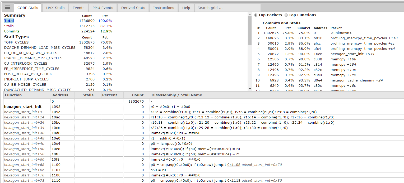
The HTML report file presents an interactive document that allows you to select and display profiling information. The CORE Stalls tab shows a Summary report, Top packets, Top Functions, the Disassembly/Stall Name, etc. In the Top Packets section, you can observe the count and percentage of the profiling packets and functions. Many of the functions shown will be internal to the Simulator. These stats give a good picture of the packets and functions running on the simulator. The other tabs available are HVX Stalls, Events, PMU Events, Derived Stats, Instructions, and Help. These tabs give additional information about the example that has been profiled.
Hexagon Trace Analyzer
Overview
The Hexagon Trace Analyzer is a software analysis tool that processes the Hexagon Embedded Trace Macrocell (ETM) traces generated by the software running on the cDSP or on the Simulator. In the instructions below, we will demonstrate how to generate a trace on the device or on the simulator when running the profiling example, and how to process this trace with the Hexagon Trace Analyzer.
Prerequisites
- The Flamegraph tool needs to be installed to $HEXAGON_SDK_ROOT/tools/debug/hexagon-trace-analyzer/ to view the results.
- The
run_profilers.pyscript installs these tools to the appropriate location when first run. - You will need an internet connection when running the script for the first time in order to download Flamegraph. The link to download this tool is given above
- The
- Flamegraph works only on systems with Perl.
- Hexagon Trace Analyzer is only supported on systems with Python 3.7.
- The Windows version of Hexagon Trace Analyzer is supported only with Python 3.7.2 AMD64.
- The Hexagon Trace Analyzer requires the modules specified in
$HEXAGON_SDK_ROOT/utils/scripts/python_requirements.txtto be installed.
NOTE Currently, profiling with HexTA is supported only on CDSP signed PD.
Setup
For the Windows version of Hexagon Trace Analyzer, Perl, Powershell and System32 must be added to the top of your PATH in Environment Variables. You can update the PATH variable as follows assuming these dependencies have been installed to their default locations:
set PATH=C:\Perl64\bin;C:\WINDOWS\system32;C:\WINDOWS\System32\WindowsPowerShell\v1.0\;%PATH%
Profile on device
The instructions below explain how to profile an application on device with the Hexagon Trace Analyzer. All these steps are automated in the walkthrough script run_profilers.py described above.
The HAP ETM framework exposes a set of APIs to enable/disable ETM tracing in a user module to trace a region of interest. Refer to HAP ETM APIs for exploring user mode ETM tracing.
- The following command configures and enables tracing on the device, and launches sysMonApp to start collecting the trace:
python $HEXAGON_SDK_ROOT/tools/debug/hexagon-trace-analyzer/target_profile_setup.py -T Target -S trace_size -O
trace_size is the size of the trace that will be collected. It is expressed in bytes, in hexadecimal format. The trace file is updated in a circular buffer so that its contents will always reflect the most recent events. The default value is 0x4000000.
The -O option retrieves all the device binaries that the Hexagon Trace Analyzer needs to parse any collected trace.
Note: The -O option is only needed the first time you run the script on a newly flashed device. It should be omitted thereafter.
- Run the application
adb wait-for-device shell export LD_LIBRARY_PATH=/vendor/lib64/:$LD_LIBRARY_PATH DSP_LIBRARY_PATH="/vendor/lib/rfsa/dsp/sdk\;/vendor/lib/rfsa/dsp/testsig;" /vendor/bin/profiling -f timers - While your application is running, copy the ETM trace to a .bin file
adb wait-for-device shell "cat /dev/coresight-tmc-etr > /data/local/tmp/trace.bin" - Copy the trace.bin to your local machine
adb wait-for-device pull /data/local/tmp/trace.bin trace.bin - Run sysMonApp to display the load offsets of all DSP libraries that were recently loaded on device
adb wait-for-device shell /data/local/tmp/sysMonApp etmTrace --command dll --q6 cdsp - You should see output lines similar to:
data.ELF_NAME = ./libsysmondomain_skel.so data.ASID = 0x00000004 data.IDENTIFIER = 0x58d0c0f0 data.LOAD_ADDRESS = 0x0836a000 data.TOKEN = 2338816 data.LOAD_TIMESTAMP = 0x000000014eae7a8b data.UNLOAD_TIMESTAMP = 0x0000000000000000 -
Start from the example config file
$HEXAGON_SDK_ROOT/examples/profiling/config_example.jsonand then replace the library names (i.e. ELF_NAME), load addresses (i.e. LOAD_ADDRESS) and ASID values (i.e. ASID) from the example config file with those obtained from the etmTrace sysMonApp service mentioned above.NOTE:
-
The ASID values are only present on recent builds on v73 and onwards
-
HexTA needs access to all the binaries that were executed during the capture of a trace in order to decode it. If HexTA misses some of these binaries, the decoding of the trace will be incomplete and thus inaccurate. It is therefore critical to list all the binaries listed by
sysMonAppand their respective load addresses. -
Make sure the LLVM_TOOLS_PATH tools version in the config.json file matches the version of the tools present in
$HEXAGON_SDK_ROOT/tools/HEXAGON_Tools/ -
If the same library name occurs multiple times with different load addresses in the report from the sysMonApp etmTrace service, include all these instances in the
config.jsonfile -
If the target is Lahaina, include
ver="V68"in the config.json file
-
-
Run the Hexagon Trace Analyzer to run generate the analysis reports:
$HEXAGON_SDK_ROOT/tools/debug/hexagon-trace-analyzer/hexagon-trace-analyzer ./config.json ./HexTA_result ./trace.bin
In the command line above
config.jsonis the configuration file you editedHexTA_resultis the directory in which the results will be placedtrace.binis the trace file that you retrieved from the device
NOTE: In rare instances, you might encounter the following error when executing HexTA:
The process cannot access the file because it is being used by another process: 'C:\\Users\\<username>\\AppData\\Local\\Temp\\hexta_ad0bw9io\\addrDict_db'
If this occurs, try re-running the profiling example after a reboot of your device. If the issue persists and your 'config.json' file contains an entry with an elf offset of 0x01000000, remove this entry from the config file before re-running HexTA. This approach will however lead to reports that are less accurate as fewer instructions will be decoded by HexTA.
Profile on simulator
The instructions below explain how to profile an application on simulator with the Hexagon Trace Analyzer. All these steps are automated in the walkthrough script run_profilers.py described above.
- Run the application on the simulator with the following args:
- --timing
- --pctrace_nano
For example to run on the DSP v66:
$DEFAULT_HEXAGON_TOOLS_ROOT/Tools/bin/hexagon-sim --timing --pctrace_nano pctrace.txt -mv66g_1024 --simulated_returnval --usefs $HEXAGON_SDK_ROOT/examples/profiling/hexagon_Debug_toolv87_v66 --pmu_statsfile $HEXAGON_SDK_ROOT/examples/profiling/hexagon_Debug_toolv87_v66/pmu_stats.txt --cosim_file $HEXAGON_SDK_ROOT/examples/profiling/hexagon_Debug_toolv87_v66/q6ss.cfg --l2tcm_base 0xd800 --rtos $HEXAGON_SDK_ROOT/examples/profiling/hexagon_Debug_toolv87_v66/osam.cfg $HEXAGON_SDK_ROOT/rtos/qurt/computev66/sdksim_bin/runelf.pbn -- $HEXAGON_SDK_ROOT/libs/run_main_on_hexagon/ship/hexagon_toolv87_v66/run_main_on_hexagon_sim -- ./$HEXAGON_SDK_ROOT/examples/profiling/hexagon_Debug_toolv87_v66/profiling_q.so -f timers
pctrace.txt using the Hexagon Simulator when running the profiling_q.so on run_main_on_hexagon_sim executable.
For other DSPs the argument -mv66g_1024 can be changed appropriately. Refer to the Running on simulator section above and simulator documentation for further information.
NOTE: Make sure in the config_simulator.json script the LLVM_TOOLS_PATH tools version is the same as $HEXAGON_SDK_ROOT/tools/HEXAGON_Tools/8.7.06 in your currently installed Hexagon SDK.
- Make sure the extension for the trace file for the simulator is .txt. If .bin is used like the trace.bin file pulled from device, the Hexagon Trace Analyzer will not be able to process the traces from simulator.
- Finally run the Hexagon Trace Analyzer with the
config_simulator.jsonfile already present in the example folder :$HEXAGON_SDK_ROOT/tools/debug/hexagon-trace-analyzer/hexagon-trace-analyzer ./config_simulator.json ./result_hexta_simulator ./pctrace.txt
In the command line above
config_simulator.jsonis the configuration fileresult_hexta_simulatoris the directory in which the results from simulator will be placedpctrace.txtis the trace file generated when running the application on the simulator
Interpreting the results
The Hexagon-Trace-Analyzer generates results in the directory specified by the user. We recommend looking at the generated files in the following order.
debug.txt
This file provides some information on the HexTA execution such as the list of elf files that were decoded and the trace decoding status. The following metrics should be reviewed each time:
-
PercentageProcessedindicates what percentage of the trace entries was successfully mapped to one of the binaries provided by the user. The higher this number, the more accurate the HexTA report will be. It is recommended to have more than 95% of the trace successfully decoded. Otherwise, look at the sysmon report to ensure all loaded binaries are listed in theconfig.jsonfile and available to HexTA. -
PHeader3CycleAccurateCountindicates whether PC cycle-accurate tracing is enabled. A value of 0 indicates that PC cycle-accurate count is not enabled and that the HexTA reports will not be accurate. Make sure that the PC cycle-accurate count is set to 1. This is done on simulator by using the-timingoption when producing a trace with the simulator. On target, cycle-accurate is enabled by default but it can also be enabled manually by running the following command prior to generating a trace:adb -s <serial number> shell /data/local/tmp/sysMonApp etmTrace --command etm --q6 cdsp --etmType ca_pcRunning
$HEXAGON_SDK_ROOT/tools/debug/hexagon-trace-analyzer/target_profile_setup.pywill execute this command.
Notes:
* The Excel files are the least affected by decoding errors occuring when HexTA does not have all binaries. This is why we recommend, after looking at debug.txt, to inspect first the contents of the Excel files before looking at the Flamegraph and Perfetto files that may be less reliable.
* Based on the symbol files provided in the HexTA configuration, some functions can be presented as hidden functions in the Perfetto traces and other views, especially when the symbol files are of .mdt extension.
perSectionStats.xlsx
This file provides an overview on how much time was spent in each code section. This may help you understand how much time was spent executing code inside a custom library versus the rest of your test.
-
perFunctionStats.xlsx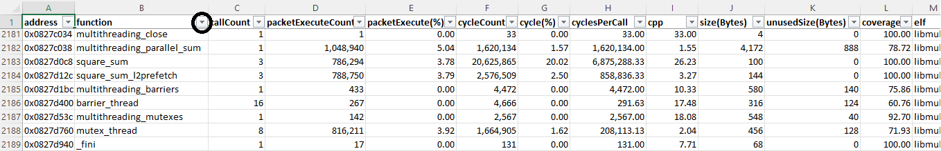
This file provides function-level information such as packet count, call count, cycle count, cpp (cycles-per-packet), function size and unused bytes.
This file may contain
hidden_functions. These entries either correspond to functions whose contents are not accessible to the end user or functions that are defined in binaries not provided by the user.If you have already identified code sections of interest, you may want to filter the per-function report by section. To do so, click on the
sectioncolumn on the first row and select or unselect sections accordingly to your choice.Similarly, you can use the drop-down filter for the
functioncolumn--circled in red in the view above--to search for functions by name.You may also sort functions by ascending or descending order for various metrics. Usually, the most useful metrics to look at are:
cycleCountorcycle(%), to identify the functions taking the most timecpp(Cycle Per Packet), to identify the functions stalling the mostcallCount, to identify the functions called the most frequently
Once you have identified the functions of interest from those metrics above, the cycle and execute count metrics are useful to understand how and why functions are stalling.
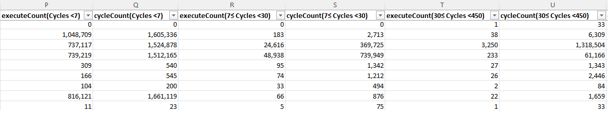
A function with a count of 20 for the
executeCount(Cycles<7)and 60cycleCount(Cycles<7)means that among all the packets this function executed, 20 Packets took less than 7 cycles to execute and these 20 packets took a total of 60 Cycles, or an average of 3 cycles per packet.executeCount(7≤ Cycles <30)reports the number of packets that took less than 30 cycles and more than 7 cycles to execute, and so on.This cycle per packet breakdown is useful to understand the types of stalls a given function incurs, and thus gives hints as to how it might be optimized further:
- packets taking between 7 and 30 cycles likely incurred L1 misses and might benefit from scalar L1 prefetches or rearchitecting your code to keep more contents (data/instruction) into L1
- packets taking between 30 and 450 cycles likely incurred L2 misses and might benefit from L2 prefetches or rearchitecting your code to keep more data into L2 or VTCM
- packets with even higher latencies may be indicative of stalls from drivers, which each have their own throughput
Do however keep in mind that packet stalls have many possible other explanations (pipeline stalls, interrupts, etc.) and that their effects may even be combined.
-
perPacketStats.xlsxOnce you have identified the functions of interest--usually the functions that consume the most cycles or the functions that stall the most (high cpp counts)--you may look at the per-packet statistics to idendify the instructions consuming the most cycles or stalling the most within each function.
To hone in on a particular function, you can use the
functiondrop-down filter.Blocks of consecutive instructions with high cycle counts are usually indicative of loop sections in which optimizations will be most beneficial to reduce the cycle count further.
As with the
perFunctionStats.xlsxyou can use thecPandcCmetrics to understand what causes some of the stalls Instructions with high cpps. -
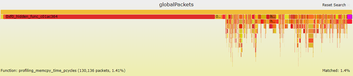
Flamegraph files
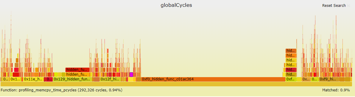
This flamegraph shows a stack trace of your profiled application, using either number of packets or number of cycles as metric. The width of each bar is proportional to the number of cycles spent in that function and its children. As a result, functions spanning over a large portion of the graph represent the functions in which the application spends the most time.
You can use the search box in the upper right corner to search functions by name within the graph. Functions matching the string being searched are highlighted in a shade of purple.
Hover over any function to obtain details about this function.
Icicle flame graphs are similar to regular flame grapahs but with an inverted layout. This inverted layout allows to identify all the callers of a given function and their respective contributions in terms of cycles or packets.
-
Perfetto files
The directory includes json files. These files represent a timeline view of the application. Long timelines are broken down in multiple files, indexed by time. Any of these files can be viewed by opening Perfetto into a Chrome browser, clicking on
Open Trace Fileand selecting the corresponding.jsonfile to view.This view shows the execution timeline on each CDSP hardware thread.
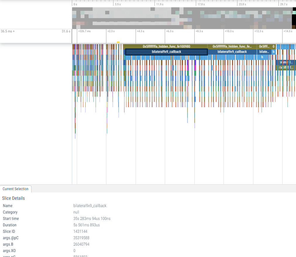
If you use the search box in Perfetto to specify a function name, the hardware thread that contains the function is highlighted. Clicking on the dropdown on that thread shows details of call-stack of the function. Clicking on the function itself shows metrics about the function in the
Current Selectionpanel, such as start time, duration, stack id, thread id , etc.The time (36.5ms) shown in the image above on the top left specifies the time since system boot and 31.6s specifies the time since the start of this .json file upto the particular time slice of interest selected.
Note A warning with the following message can be safely ignored : "Perfetto UI features are limited for JSON traces. We recommend recording proto-format traces from Chrome."
-
Run command using the
run_profilers.pyscript: -
For device:
python run_profilers.py -T lahaina -HT -
For simulator:
python run_profilers.py -HS
Running the script will generate the following files:
| File name | Description | Notes |
|---|---|---|
| trace.bin | Trace file of the profiled application | Pulled from the device |
| *.svg | Stack trace of the profiled application | Generated with Flamegraph and viewed in a browser offline |
| *.json | Timeline showing function activity per thread | Viewed with Perfetto viewer offline |
| *.xlsx | Instruction- or function-level cycle and stall analysis | Viewed with Excel |
On the Perfetto interface, you can pan and zoom, in and out of the graphical representation using the keys w to zoom in, s to zoom out, d to pan right, and a to pan left. You can search for functions in the Search box at the top of the page. The statistics of a selected function appear in the bottom half of the page.
Note: The Hexagon Trace Analyzer traces are organized as follows:
hwt_perfetto*.jsonfiles only contain the hardware thread activityperfetto*.jsonfiles contain:- CPP metric
- hardware thread activity
- function activity
Furthermore, the JSON files are split to represent successive blocks of time. This allows the browser to load each JSON file more quickly.
Results obtained on simulator are quite similar to those obtained when obtaining a trace from the device.
Known Limitations
-
Tracing software threads on the simulator is not supported, hence it is not possible to derive a per software thread callstack for the Flamegraph or Perfetto outputs.
-
The time unit for traces captured on the simulator can only be pcycles. The time (us) unit is only supported when running on device.
sysMonApp
Overview
The sysMonApp is an app that configures and displays multiple performance-related services on the cDSP, aDSP, and sDSP. The sysMonApp can be run as a standalone profiling tool or as an Android Application. In the instructions below we will demonstrate how to use the sysMonApp profiler tools to analyze the profiling example on the device.
Profile from the Command Line
- Copy the sysMonApp to the device
adb push $HEXAGON_SDK_ROOT/tools/utils/sysmon/sysMonApp /data/local/tmp/ adb shell chmod 777 /data/local/tmp/sysMonApp - Make sure adsprpcd is running:
adb shell ps | grep adsprpcd - Run the sysMonApp profiler service in user mode on cDSP as follows:
adb shell /data/local/tmp/sysMonApp profiler --debugLevel 1 --q6 cdsp - Run the profiling example on device:
adb wait-for-device shell export LD_LIBRARY_PATH=/vendor/lib64/:$LD_LIBRARY_PATH DSP_LIBRARY_PATH="/vendor/lib/rfsa/dsp/sdk\;/vendor/lib/rfsa/dsp/testsig;" /vendor/bin/profiling -f inbuf -s 65536 -m') -
The previous command should have generated a file
/sdcard/sysmon_cdsp.bin. This file should be pulled to your local computer as follows:NOTE: On some devices, the trace file may be generated in the /data folder instead.adb pull /sdcard/sysmon_cdsp.bin -
The
sysmon_cdsp.binfile can be parsed with the sysMonApp parser service as shown below. -
Run the sysMonApp Parser
NOTE: The Hexagon SDK contains Windows and Linux versions of the parser. Both versions have the same interface. Below we illustrate how to use the Linux parser. For Windows simply replace parser_linux_v2 with parser_win_v2 in the commands below.
- The following example command shows how to generate HTML and CSV files in Linux to output directory
sysmon_parsed_output. The sysMonApp parser usage can be found here. The Windows tool expects the same arguments:$HEXAGON_SDK_ROOT/tools/utils/sysmon/parser_linux_v2/HTML_Parser/sysmon_parser ./sysmon_cdsp.bin --outdir sysmon_parsed_output
Profile using Android Application
- Install the sysMon DSP profiler application on the device using adb install:
adb install -g $HEXAGON_SDK_ROOT/tools/utils/sysmon/sysMon_DSP_Profiler_V2.apk - The sysMon DSP Profiler UI for the sysMonApp Android Application provides user flexibility to choose from different modes of profiling. You can select the Mode based on your requirements. The available modes are:
| Mode | Description |
|---|---|
| DSP DCVS | User can adjust DSP core and bus clocks dynamically for profiling duration. |
| Default Mode | A fixed set of performance metrics will be monitored. Sampling period is either 1 or 50 milli-seconds. |
| User Mode | If Default Mode is unchecked, User Mode is enabled. The user can select the desired PMU events to be captured. |
| 8-PMU Mode | If both DSP DCVS and Default modes are unchecked, 8-PMU mode is enabled. This allows user to choose whether to configure 4 PMU events or 8 PMU Events. |
- The Configuration Settings button is enabled in user mode and you can select the PMU events to be captured.
- Further details about the different modes and options can be found in sysMonApp Profiler.
Understanding the results
- The files generated by sysMon Profiler application are the following:
| File name | Description |
|---|---|
| sysmon_cdsp.bin | This is the cDSP binary file pulled from the device. |
| sysmon_report directory | This directory is generated after running the sysMonApp HTML Parser. It contains HTML and csv files generated by the HTML Parser. This directory is named based on the date the report was generated. |
- The sysMonApp HTML file gives an overall summary of the profiling done using the sysMonApp. Here is an example of the HTML generated from the sysMonApp.
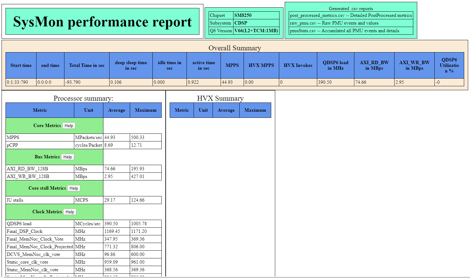
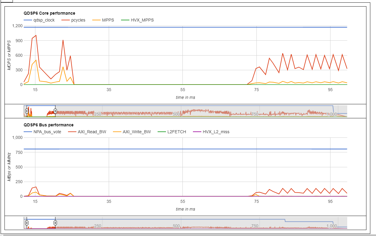
- To understand the output of these files generated please refer to the sysMonApp profiler documentation